Backpropagating Through Time Itself: Reverse-Mode Autodiff of ODE Solutions

Most neural networks are built out of layers. You stack them, you count them, and the number is an integer: 12 layers, 50 layers, 175 layers. In 2018 a group of researchers at the University of Toronto asked an odd question — what if the number of layers were a real number? What if depth were continuous?

That question turned a neural network into a differential equation. And it created a very concrete problem: if your model is an ODE solver, how do you backpropagate through it?

This post builds up to the answer. We'll start with what an ODE is, look at how solvers actually work, see why naive backpropagation through a solver is a bad idea, and then walk carefully through the adjoint sensitivity method — the technique that computes exact gradients while using essentially no memory.

What is an ODE?
How ODE solvers actually work
Why machine learning cares: from ResNets to Neural ODEs
The training problem
The adjoint sensitivity method
Reading the diagram
The full backward algorithm
Why does the adjoint ODE look like that?
Costs, trade-offs, and things that bite
A minimal implementation
Takeaways
References

1. What is an ODE?

An ordinary differential equation is an equation that describes change rather than value. Instead of telling you where something is, it tells you how fast it's moving, and leaves you to figure out the rest.

The general form we care about is:

\frac{d\mathbf{z}(t)}{dt} = f(\mathbf{z}(t), t, \theta)

Read it out loud: the rate of change of the state $\mathbf{z}$ at time $t$ is some function $f$ of the current state, the current time, and some parameters $\theta$ .

The pieces:

Symbol	Meaning
$\mathbf{z}(t)$	the state — a vector describing the system at time $t$
$t$	the independent variable, usually time
$f$	the dynamics or vector field — the rule for how the state changes
$\theta$	parameters of the dynamics

"Ordinary" just means there's a single independent variable ( $t$ ). If the state also varied over space and you had derivatives in multiple directions, you'd have a partial differential equation, which is a harder story.

The initial value problem

An ODE on its own doesn't have a unique solution. "The car is moving at 60 km/h" doesn't tell you where the car is — you also need to know where it started. Pair the ODE with a starting condition $\mathbf{z}(t_0)$ and you get an initial value problem (IVP), which (under mild smoothness conditions) has exactly one solution.

Solving an IVP means integrating:

\mathbf{z}(t_1) = \mathbf{z}(t_0) + \int_{t_0}^{t_1} f(\mathbf{z}(t), t, \theta)\, dt

This is the key mental shift. An ODE is a local rule; a solution is a global trajectory. The dynamics $f$ tells you which way to step at every point; the solution is the path you trace out by following those instructions from a starting point.

A concrete example

Take population growth where the growth rate is proportional to the current population:

\frac{dz}{dt} = kz, \qquad z(0) = z_0

This one has a closed-form solution: $z(t) = z_0 e^{kt}$ . Exponential growth falls out of a one-line local rule.

But closed-form solutions are the exception, not the rule. The vast majority of ODEs that describe anything interesting — orbital mechanics, chemical kinetics, epidemiology, fluid flow — have no analytic solution at all. For those, we integrate numerically.

2. How ODE solvers actually work

A numerical ODE solver answers a simple question repeatedly: given where I am now and which way the field points, where should I be a moment from now?

The simplest possible answer is Euler's method: pretend the derivative is constant over a small step $\Delta t$ .

\mathbf{z}_{n+1} = \mathbf{z}_n + \Delta t \cdot f(\mathbf{z}_n, t_n, \theta)

Step, evaluate, step, evaluate — until you reach $t_1$ .

flowchart TD
    A(["start: z = z(t₀), t = t₀"]) --> B["evaluate the dynamics<br/>f(z, t, θ)"]
    B --> C["take a step<br/>z ← z + Δt · f"]
    C --> D["advance time<br/>t ← t + Δt"]
    D --> E{"t ≥ t₁ ?"}
    E -->|no| B
    E -->|yes| F(["return z(t₁)"])

    classDef term fill:#2a0f18,stroke:#e11d48,stroke-width:1.5px,color:#fda4af;
    class A,F term;

Euler's method is easy to understand and not very good. The error per step scales with $\Delta t^2$ , so you need tiny steps for decent accuracy. Real solvers do something smarter:

Runge–Kutta 4 (RK4) evaluates $f$ four times per step at cleverly chosen intermediate points and blends the results, achieving far higher accuracy for the same step size.
Adaptive solvers (Dormand–Prince, dopri5) estimate their own error at each step and shrink or grow $\Delta t$ automatically. Smooth regions get big steps; violent regions get small ones.
Implicit / stiff solvers (BDF, Radau) handle systems where some components change vastly faster than others and explicit methods would need absurdly tiny steps.

Two properties matter enormously for what follows:

The number of steps is not fixed in advance. An adaptive solver decides at runtime how many times to call $f$ . It might be 20 calls, it might be 2,000.
Every step is a differentiable operation. Each one is just arithmetic on the output of $f$ .

That second point is what makes the naive approach tempting — and the first is what makes it painful.

3. Why machine learning cares: from ResNets to Neural ODEs

Here's the observation that started all this. A residual network layer computes:

\mathbf{h}_{t+1} = \mathbf{h}_t + f(\mathbf{h}_t, \theta_t)

Compare that to an Euler step with $\Delta t = 1$ :

\mathbf{z}_{n+1} = \mathbf{z}_n + \Delta t \cdot f(\mathbf{z}_n, t_n, \theta)

They're the same equation. A ResNet is a crude ODE solver running on a learned vector field. Each residual block is one clumsy Euler step through a dynamical system.

So instead of stacking discrete blocks, parameterise the derivative directly with a neural network and hand the whole thing to a real solver:

\frac{d\mathbf{z}(t)}{dt} = f(\mathbf{z}(t), t, \theta), \qquad \mathbf{z}(t_1) = \text{ODESolve}(\mathbf{z}(t_0), f, t_0, t_1, \theta)

flowchart TB
    subgraph RES["ResNet · discrete depth"]
        r0(["h₀"]) --> r1["h₁ = h₀ + f(h₀, θ₀)"]
        r1 --> r2["h₂ = h₁ + f(h₁, θ₁)"]
        r2 --> r3(["h₃ = h₂ + f(h₂, θ₂)"])
    end
    subgraph ODE["Neural ODE · continuous depth"]
        o0(["z(t₀)"]) --> o1["dz/dt = f(z, t, θ)<br/>one shared network"]
        o1 -->|"the solver decides how<br/>many evaluations to make"| o2(["z(t₁)"])
    end

    classDef term fill:#2a0f18,stroke:#e11d48,stroke-width:1.5px,color:#fda4af;
    class r0,r3,o0,o2 term;

The payoff is real: constant parameter count regardless of "depth", a natural way to model irregularly-sampled time series, an explicit accuracy/compute dial you can turn at inference time, and invertible dynamics that make continuous normalising flows tractable.

But now the forward pass of your model is a numerical integration routine. Which brings us to the hard part.

4. The training problem

Training needs $\partial L / \partial \theta$ . The obvious approach: the solver is made of differentiable operations, so just record them all on the autodiff tape and backpropagate through the solver's internals.

This works. It's also a bad idea, for three reasons:

Memory. You must store every intermediate state and every intermediate activation inside every evaluation of $f$ . With an adaptive solver taking hundreds of steps, memory grows linearly with the number of function evaluations — and you don't know that number until runtime. Depth is now a memory liability, exactly the thing continuous-depth models were supposed to escape.

Numerical error accumulation. You're differentiating the approximation the solver produced, not the true solution. Errors introduced by the discretisation get baked into the gradient.

Solver coupling. Your gradient computation is welded to the internals of one specific solver. Swap dopri5 for an implicit method and you have to differentiate through a nonlinear root-find.

What we want instead: treat the solver as a black box, and get gradients some other way.

5. The adjoint sensitivity method

The trick, which goes back to Pontryagin's work on optimal control in 1962, is to compute gradients by solving a second ODE backwards in time.

Start with the loss. Its input is the output of an ODE solver:

L(\mathbf{z}(t_1)) = L\left(\mathbf{z}(t_0) + \int_{t_0}^{t_1} f(\mathbf{z}(t), t, \theta)\, dt\right) = L\big(\text{ODESolve}(\mathbf{z}(t_0), f, t_0, t_1, \theta)\big) \tag{3}

To optimise $L$ we need gradients with respect to $\theta$ . The first step is to work out how the gradient of the loss depends on the hidden state at each instant. That quantity is called the adjoint:

\mathbf{a}(t) = \frac{\partial L}{\partial \mathbf{z}(t)}

Read that carefully: $\mathbf{a}(t)$ is the sensitivity of the final loss to a perturbation of the state at time $t$ . If you nudged the trajectory at time $t$ , how much would the loss move? It's the continuous-time analogue of the gradient signal that flows backwards through a ResNet — except instead of one vector per layer, it's a vector-valued function of continuous time.

And here is the beautiful part: the adjoint obeys its own ODE.

\frac{d\mathbf{a}(t)}{dt} = -\mathbf{a}(t)^{\mathsf{T}} \frac{\partial f(\mathbf{z}(t), t, \theta)}{\partial \mathbf{z}} \tag{4}

This is the instantaneous analogue of the chain rule. In discrete backprop you multiply by a Jacobian at each layer; here you integrate against a Jacobian continuously. The minus sign is the tell — it means this equation is naturally solved backwards in time.

So we can compute $\partial L / \partial \mathbf{z}(t_0)$ with another call to an ODE solver, running from $t_1$ back to $t_0$ , starting from the known value $\partial L / \partial \mathbf{z}(t_1)$ .

One complication: equation (4) needs $\mathbf{z}(t)$ along the whole trajectory, and we deliberately threw that away. The fix is elegant — recompute $\mathbf{z}(t)$ backwards alongside the adjoint, starting from its final value $\mathbf{z}(t_1)$ . The original ODE runs just as happily in reverse.

Finally, the parameter gradients require a third integral, one that depends on both $\mathbf{z}(t)$ and $\mathbf{a}(t)$ :

\frac{dL}{d\theta} = -\int_{t_1}^{t_0} \mathbf{a}(t)^{\mathsf{T}} \frac{\partial f(\mathbf{z}(t), t, \theta)}{\partial \theta}\, dt \tag{5}

Intuitively: at every instant, the parameters nudged the vector field by $\partial f / \partial \theta$ , and the loss cared about state perturbations at that instant by $\mathbf{a}(t)$ . Multiply and accumulate over the whole trajectory.

Three quantities, three coupled ODEs, one backwards solve. That's the whole method.

6. Reading the diagram

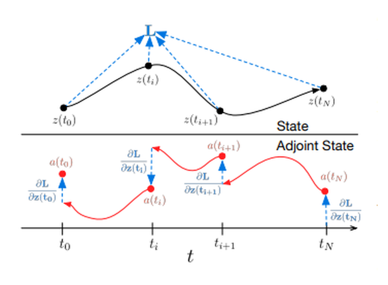
Two stacked plots sharing a time axis from t₀ to t_N. The upper panel shows the forward state trajectory z(t) as a black curve with observation points, each connected by dashed blue arrows to the loss L above. The lower panel shows the adjoint state a(t) as a red curve flowing backwards in time, with vertical blue arrows marking discrete jumps of size ∂L/∂z at each observation time.

Figure 1. Reverse-mode differentiation of an ODE solution. The adjoint sensitivity method solves an augmented ODE backwards in time. The augmented system carries both the original state and the sensitivity of the loss to that state. When the loss depends directly on the state at several observation times, the adjoint must be updated in the direction of the partial derivative of the loss with respect to each observation. (Reproduced from Chen et al., 2018, Figure 2 — see references.)

This single figure contains the entire method. Let's take it apart.

The shared time axis

Both panels sit on the same horizontal axis, running from $t_0$ on the left to $t_N$ on the right, with observation times $t_i$ and $t_{i+1}$ in between. Everything in the figure is happening over the same interval — the two panels are two different things travelling across the same stretch of time, in opposite directions.

Upper panel — the forward pass (state)

The black curve is $\mathbf{z}(t)$ , the solution trajectory, integrated left to right from $\mathbf{z}(t_0)$ to $\mathbf{z}(t_N)$ . The black dots mark the times at which we actually observe the state and evaluate the loss.

The dashed blue arrows all converge upward on $L$ . That's the figure telling you something important: the loss doesn't only depend on the endpoint. In a time-series setting you compare predictions to data at many timestamps, so $\mathbf{z}(t_i)$ , $\mathbf{z}(t_{i+1})$ and $\mathbf{z}(t_N)$ each contribute their own term to $L$ . Each arrow is one such contribution.

Lower panel — the backward pass (adjoint)

The red curve is $\mathbf{a}(t) = \partial L / \partial \mathbf{z}(t)$ , and it flows right to left. Note the direction of the red arrowheads — they point backwards along the axis, from $t_N$ toward $t_0$ . This is equation (4) being solved in reverse time. The adjoint is born at $t_N$ , from the loss, and propagates backwards to $t_0$ , arriving as $\partial L / \partial \mathbf{z}(t_0)$ — the gradient with respect to the input.

Between observations, the red curve is smooth: it's just following its ODE, sliding continuously as the Jacobian $\partial f/\partial \mathbf{z}$ reshapes it.

The vertical blue arrows — the crucial detail

At each observation time you'll see a short vertical blue arrow labelled $\frac{\partial L}{\partial \mathbf{z}(t_i)}$ . These are discontinuous jumps in the adjoint, and they're the part people miss on a first read.

Here's why they exist. The adjoint accumulates all the ways the state at time $t$ influences the loss. Just to the right of $t_i$ , that influence is entirely indirect — the state at $t_i^+$ affects the loss only by propagating forward through the dynamics to later observations. But at $t_i$ itself, a new direct path opens up: $\mathbf{z}(t_i)$ appears explicitly in the loss via its own data term.

So as the backward integration arrives at an observation time, you must add that direct contribution:

\mathbf{a}(t_i^-) = \mathbf{a}(t_i^+) + \frac{\partial L}{\partial \mathbf{z}(t_i)}

Skip this and your gradients are silently wrong — the model will train, badly, and you'll spend a week blaming the learning rate. If the loss depends only on the final state $\mathbf{z}(t_1)$ , there's exactly one such jump: the one that initialises the adjoint at $t_1$ .

The one-sentence summary of the figure

The state flows forward through time and feeds the loss; the adjoint flows backward through time and collects gradient, jumping discontinuously every time it passes a point where the loss touched the trajectory directly.

7. The full backward algorithm

We now have three things to compute backwards: the state $\mathbf{z}(t)$ , the adjoint $\mathbf{a}(t)$ , and the running parameter-gradient integral $\partial L / \partial \theta$ . Rather than three separate solves, stack them into a single augmented state:

\mathbf{s}(t) = \big[\, \mathbf{z}(t),\; \mathbf{a}(t),\; \tfrac{\partial L}{\partial \theta} \,\big]

with augmented dynamics:

\frac{d\mathbf{s}}{dt} = \left[\, f(\mathbf{z}, t, \theta),\; -\mathbf{a}^{\mathsf{T}}\frac{\partial f}{\partial \mathbf{z}},\; -\mathbf{a}^{\mathsf{T}}\frac{\partial f}{\partial \theta} \,\right]

Then call the same black-box solver on this bigger system, running from $t_1$ to $t_0$ . One backwards solve produces everything.

flowchart TD
    A["FORWARD<br/>solve dz/dt = f from t₀ to t₁"] --> B["keep only z(t₁)<br/>discard the trajectory"]
    B --> C["evaluate the loss L<br/>compute ∂L/∂z(t₁)"]
    C --> D["initialise the augmented state at t₁<br/>s = ⟨ z(t₁), ∂L/∂z(t₁), 0 ⟩"]
    D --> E["BACKWARD<br/>integrate the augmented ODE<br/>z, a and the θ-gradient evolve together"]
    E --> F{"reached an<br/>observation time tᵢ ?"}
    F -->|yes| G["jump the adjoint<br/>a ← a + ∂L/∂z(tᵢ)"]
    G --> E
    F -->|"no — arrived at t₀"| H["read off the results<br/>∂L/∂z(t₀) and dL/dθ"]
    H --> I(["optimiser step on θ"])

    classDef phase fill:#2a0f18,stroke:#e11d48,stroke-width:1.5px,color:#fda4af;
    class A,E,I phase;

Written as pseudocode:

def adjoint_backward(z_t1, dL_dz_t1, t0, t1, theta, f):
    # Augmented state: (state, adjoint, parameter-gradient accumulator)
    s0 = (z_t1, dL_dz_t1, zeros_like(theta))

    def aug_dynamics(s, t):
        z, a, _ = s
        # One vector-Jacobian product gives every Jacobian we need.
        # We never form the Jacobian matrices explicitly.
        df_dz, df_dtheta = vjp(f, (z, t, theta), v=a)
        return (f(z, t, theta), -df_dz, -df_dtheta)

    # Same black-box solver as the forward pass, integrated in reverse
    z_t0, dL_dz_t0, dL_dtheta = ODESolve(s0, aug_dynamics, t1, t0)
    return dL_dz_t0, dL_dtheta

Two implementation notes worth internalising:

No Jacobians are ever materialised. The terms $\mathbf{a}^{\mathsf{T}} \partial f/\partial \mathbf{z}$ and $\mathbf{a}^{\mathsf{T}} \partial f/\partial \theta$ are vector–Jacobian products, exactly what reverse-mode autodiff computes natively. One vjp call through $f$ with cotangent $\mathbf{a}$ gives you both. Cost is comparable to evaluating $f$ itself.
Autodiff is still used — just locally. We backpropagate through a single evaluation of $f$ , never through the solver's step-taking machinery. That's the whole memory saving.

8. Why does the adjoint ODE look like that?

A quick sketch of where equation (4) comes from, for readers who want the mechanism rather than the assertion.

Consider two nearby times $t$ and $t + \varepsilon$ . The state at $t + \varepsilon$ is determined by the state at $t$ :

\mathbf{z}(t + \varepsilon) = \mathbf{z}(t) + \int_t^{t+\varepsilon} f(\mathbf{z}(\tau), \tau, \theta)\, d\tau \approx \mathbf{z}(t) + \varepsilon f(\mathbf{z}(t), t, \theta)

The chain rule links the sensitivities at the two times:

\mathbf{a}(t) = \mathbf{a}(t+\varepsilon)^{\mathsf{T}} \frac{\partial \mathbf{z}(t+\varepsilon)}{\partial \mathbf{z}(t)}

Substituting the expansion, that Jacobian is $\mathbf{I} + \varepsilon \frac{\partial f}{\partial \mathbf{z}} + \mathcal{O}(\varepsilon^2)$ , so:

\mathbf{a}(t) \approx \mathbf{a}(t+\varepsilon)^{\mathsf{T}}\left(\mathbf{I} + \varepsilon \frac{\partial f}{\partial \mathbf{z}}\right)

Rearranging into a difference quotient and letting $\varepsilon \to 0$ gives exactly equation (4). The negative sign appears because $\mathbf{a}(t)$ is being expressed in terms of $\mathbf{a}$ at a later time — information moves backwards.

Notice what this means structurally: standard backprop through a ResNet does $\mathbf{a} \leftarrow \mathbf{a}(\mathbf{I} + \partial f/\partial \mathbf{z})$ once per block. The adjoint ODE does the same thing in the limit of infinitely many infinitesimal blocks. It is backpropagation, taken continuously.

9. Costs, trade-offs, and things that bite

	Backprop through solver	Adjoint method
Memory	$\mathcal{O}(\text{number of function evals})$	$\mathcal{O}(1)$ in solver steps
Compute	~1 forward + 1 backward tape	~1 forward + 1 backward solve (roughly 2×)
Gradient exactness	Exact w.r.t. the discretised solution	Exact w.r.t. the true solution, up to reverse-solve tolerance
Solver independence	Coupled to internals	Fully black-box
Scaling with depth	Linear memory growth	Flat

The headline win is memory: constant cost regardless of how many steps the solver decides to take. That's what makes continuous-depth models trainable at all.

The honest caveats:

Reverse-recomputation drift. Recovering $\mathbf{z}(t)$ by integrating backwards from $\mathbf{z}(t_1)$ is not bit-identical to the forward trajectory. For chaotic or stiff dynamics the two can diverge meaningfully, corrupting gradients. Remedies include tighter reverse tolerances, checkpointing a handful of intermediate states, or reversible/symplectic solvers.
NFE creep. As training progresses the learned vector field often becomes stiffer, and adaptive solvers respond by taking more steps. Number-of-function-evaluations climbs, and wall-clock time with it. Regularising the dynamics toward smoothness helps.
Roughly 2× compute. You're trading time for memory. Sometimes that's the wrong trade — for short integrations with few steps, plain backprop through the solver can be both simpler and faster.
Don't forget the jumps. As stressed above, multi-observation losses need the adjoint updated at every observation time. Good libraries handle this; hand-rolled implementations frequently don't.

10. A minimal implementation

In PyTorch with torchdiffeq, the entire method is one import swap:

import torch
import torch.nn as nn
from torchdiffeq import odeint_adjoint as odeint   # <- adjoint method
# from torchdiffeq import odeint                   # <- backprop through solver

class ODEFunc(nn.Module):
    """Parameterises dz/dt = f(z, t, θ)."""
    def __init__(self, dim=2, hidden=64):
        super().__init__()
        self.net = nn.Sequential(
            nn.Linear(dim + 1, hidden), nn.Tanh(),
            nn.Linear(hidden, hidden),  nn.Tanh(),
            nn.Linear(hidden, dim),
        )

    def forward(self, t, z):
        t_vec = t.expand(z.shape[0], 1)
        return self.net(torch.cat([z, t_vec], dim=-1))


func = ODEFunc()
opt = torch.optim.Adam(func.parameters(), lr=1e-3)

z0 = torch.randn(32, 2)
t = torch.linspace(0., 1., 20)          # observation times
target = torch.randn(20, 32, 2)         # stand-in for real data

for step in range(1000):
    opt.zero_grad()
    pred = odeint(func, z0, t, rtol=1e-5, atol=1e-7)   # (len(t), batch, dim)
    loss = ((pred - target) ** 2).mean()
    loss.backward()      # runs the augmented backward solve
    opt.step()

That loss.backward() call is doing everything in section 7: initialising the augmented state, integrating it backwards, applying the adjoint jumps at each of the 20 observation times, and depositing .grad on every parameter. Switching between the two imports changes memory profile and gradient semantics while leaving the training loop untouched — a useful A/B test to run on your own problem before committing.

11. Takeaways

An ODE specifies how a state changes; solving it means integrating that local rule into a global trajectory.
A ResNet is an Euler solver in disguise. Replace the discrete stack with a learned vector field and a real solver, and depth becomes continuous.
Backpropagating through the solver's internals costs memory linear in the number of steps — which defeats the purpose and depends on runtime decisions you can't predict.
The adjoint $\mathbf{a}(t) = \partial L/\partial \mathbf{z}(t)$ satisfies its own ODE. Solve it backwards in time and you get input gradients; integrate one more term along the way and you get parameter gradients.
Bundle state, adjoint and parameter-gradient into one augmented system, hand it to the same black-box solver in reverse, and you get exact gradients at constant memory.
At every time the loss touches the trajectory directly, the adjoint jumps by $\partial L/\partial \mathbf{z}(t_i)$ . That's what the vertical blue arrows in the figure are telling you.

Backpropagation was never really about layers. It's about propagating sensitivity backwards along a computation. Make the computation continuous, and backpropagation becomes a differential equation.

12. References

Chen, R. T. Q., Rubanova, Y., Bettencourt, J., & Duvenaud, D. (2018). Neural Ordinary Differential Equations. Advances in Neural Information Processing Systems 31 (NeurIPS 2018). arXiv:1806.07366. — arxiv.org/abs/1806.07366 Primary source for this post. Section 2 and Figure 2 (reproduced above as Figure 1) are the basis of the discussion of reverse-mode differentiation of ODE solutions. Winner of the NeurIPS 2018 Best Paper Award.
Pontryagin, L. S., Boltyanskii, V. G., Gamkrelidze, R. V., & Mishchenko, E. F. (1962). The Mathematical Theory of Optimal Processes. Interscience Publishers. Original development of the adjoint sensitivity method in the context of optimal control.
Chen, R. T. Q. torchdiffeq: Differentiable ODE solvers with full GPU support and O(1)-memory backpropagation. — github.com/rtqichen/torchdiffeq
Kidger, P. (2022). On Neural Differential Equations. PhD thesis, University of Oxford. arXiv:2202.02435. — arxiv.org/abs/2202.02435 Comprehensive modern treatment, including a careful discussion of when the adjoint method's gradients degrade.
Kilcher, Y. (2019). Neural Ordinary Differential Equations. Video walkthrough by Yannic Kilcher, YouTube. — youtube.com/watch?v=jltgNGt8Lpg Narrated read-through of reference 1 — a useful companion if you'd rather hear the paper explained than read it.